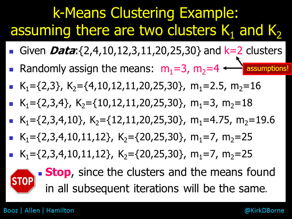
In a related post we discussed the Cold Start Problem in Data Science — how do you start to build a model when you have either no training data or no clear choice of model parameters. An example of a cold start problem is k-Means Clustering, where the number of clusters k in the data set is not known in advance, and the locations of those clusters in feature space (i.e., the cluster means) are not known either. So, you start by assuming a value for k and making random assumptions about the cluster means, and then iterate until you find the optimal set of clusters, based upon some evaluation metric. See the related post for more details about the cold start challenge. See the attached graphic below for a simple demonstration of a k-Means Clustering application.

The above example (clustering) is taken from unsupervised machine learning (where there are no labels on the training data). There are also examples of cold start in supervised machine learning (where you do have class labels on the training data).

As an example of a cold start in supervised learning, we look at neural network models, where the weights on the edges that connect the various nodes in the network layers are not known initially. So, random values (e.g., all weights = 1) are assigned to all of the edge weights (which could number in the hundreds or thousands) — that’s the cold start. Following that, the weights can “learn” to get better through a technique known as backpropagation, which is applied through sequential iterations of the neural network learning process. A validation metric estimates the error in each model iteration in the sequence (i.e., the classification error on the validation or hold-out data set), then applies the backpropagation technique to assign some portion of the error to each of the edge weights. Each edge weight is adjusted accordingly using gradient descent (or some similar error correction rate estimator) for the next model in the sequence. The next iteration of the neural network modeling process is executed, applying the same steps as above, and the process continues until the validation metric converges to the optimal final model.

What is missing in the above discussion is the deeper set of unknowns in the learning process. This is the meta-learning phase. We can elucidate this phase through our two examples above.

From the first example above, k-Means Clustering:

• What is the value of k?
• Which features in the data set are most effective in creating distinct clusters in the data (i.e., to create the segments that are the most compact internally, and relatively the most separated from each other)? There might be dozens or hundreds or thousands of attributes to choose from, and a vast number of combinations of those attributes in which to explore clustering in different dimensions of parameter space.
• What distance metric should be used to estimate separation (or what similarity metric should be used to estimate similarity), since clustering is a distance-based algorithm? There are some common choices for distance and similarity metrics (e.g., cosine similarity, Euclidean distance, Manhattan distance, Mahalanobis distance, Lp-Norm, etc.), but that is just the tip of a vast iceberg — just take a look at the 750-page book “Encyclopedia of Distances“.
• What evaluation metric should we use to determine if the clusters are “good enough” or optimal (i.e., the most compact set of clusters relative to the separation of the clusters)? There are several choices for such evaluation metrics: Dunn index, Davies-Bouldin index, C-index, and Silhouette analysis are just a few examples.

We need to decide on all of these parameterizations of the clustering model before the cold start interations on the cluster means can begin.

From the second example above, Neural Network modeling, there are also many different preliminary tasks and parameterizations of the network that need to be decided and acted on before the cold start iterations on the edge weights can begin:

• How will we measure the supervised learning model’s accuracy? e.g., true positive rate, true negative rate, total accuracy, F1-score, or what?
• How many hidden layers should there be?
• How many nodes should there be in each hidden layer?
• Which input features (explanatory variables), or engineered combinations of those variables, should we use in the input layer?
• What activation function should we use?
• There are still more choices, as shown in the list of 24 neural network adjustments, which includes architecture and hyperparameter tuning.

This now gets to the heart of meta-learning. It is focused on learning the right tasks to perform and on tuning the modeling hyper-parameters. These are the different tasks and “external” parameters that differentiate various instantiations of a specific model within a broader category of models — those tasks and external parameterizations must be explored before you start building, iterating, and validating a specific model’s “internal” parameters. For example:

• You can cluster children’s toys in a toy store by color, or by shape, or by electronic vs. non-electronic, or by age-appropriateness, or by functionality, or cluster them by some combination of those features.
• You can cluster (segment) your customers by the types of products they buy, or by their geographic location, or by their gender, or by their age, or by the day of week that they prefer to shop, or cluster them by some combination of those many different variables.
• You can cluster medical drug treatments by the types of symptoms that they address, or by the medical diagnoses (outcomes) that they attempt to cure, or by their dosage amounts, or cluster them by the side-effects that are caused when different combinations of the drugs are used.

Deciding on the higher-level hyper-parameterizations of your clustering approach before you build the actual models is good data science and good business, no matter whether you are sorting toys, or discovering segments in your customer database, or prescribing different medications to medical patients.

Similar decisions must be made for the neural network example mentioned earlier as well as for numerous other machine learning modeling techniques. Meta-learning is important to make sure that you are aware of and attentive to the many choices of modeling tasks and parameterizations for the models that you are about to train. Meta-learning is also critical for demonstrating (proving) that you built the best (or optimal or most accurate) model, given the higher level characteristics (e.g., parameters, architecture, or input data sources) of the modeling effort:

• What is the business case? What outcomes will be actionable?
• What data do we have? Which combinations of data have we not explored yet?
• What metric will demonstrate that we have achieved the globally optimal model (or approximately the global optimum), versus some locally good model that doesn’t generalize across a larger data set?

Genetic Algorithms (GAs) are an example of meta-learning. They are not machine learning algorithms in themselves, but GAs can be applied across ensembles of machine learning models and tasks, in order to find the optimal model (perhaps globally optimal model) across a collection of locally optimal solutions.

Learn more about meta-learning from these resources:

• “From zero to research — An introduction to Meta-learning“
• “What’s New in Deep Learning Research: Understanding Meta-Learning“
• “Learning to Learn“
• Meta Learning presentation
• Workshop on Meta-Learning (MetaLearn 2018)

Finally, in addition to the awesome 750-page book “Encyclopedia of Distances“, please check out some of these top-selling books on Data Science, AI, and Machine Learning:

Top Books in AI and Machine Learning

Disclosure statement: As an Amazon Associate I earn from qualifying purchases.