The ancient philosopher Confucius has been credited with saying “study your past to know your future.” This wisdom applies not only to life but to machine learning also. Specifically, the availability and application of labeled data (things past) for the labeling of previously unseen data (things future) is fundamental to supervised machine learning.

Without labels (diagnoses, classes, known outcomes) in past data, then how do we make progress in labeling (explaining) future data? This would be a problem.

A related problem also arises in unsupervised machine learning. In these applications, there is no requirement or presumption regarding the existence of labeled training data — we are essentially parameterizing or characterizing the patterns in the data (e.g., the trends, correlations, segments, clusters, associations).

Many unsupervised learning models can converge more readily and be more valuable if we know in advance which parameterizations are best to choose. If we cannot know that (i.e., because it truly is unsupervised learning), then we would like to know at least that our final model is optimal (in some way) in explaining the data.

In both of these applications (supervised and unsupervised machine learning), if we don’t have these initial insights and validation metrics, then how does such model-building get started and get moving towards the optimal solution?

This challenge is known as the cold-start problem! The solution to the problem is easy (sort of): We make a guess — an initial guess! Usually, that would be a totally random guess.

That sounds so… so… random! How do we know whether it’s a good initial guess? How do we progress our model (parameterizations) from that random initial choice? How do we know that our progression is moving towards more accurate models? How? How? How?

This can be a real challenge. Of course nobody said the “cold start” problem would be easy. Anyone who has ever tried to start a very cold car on a frozen morning knows the pain of a cold start challenge. Nothing can be more frustrating on such a morning. But, nothing can be more exhilarating and uplifting on such a morning than that moment when the engine starts and the car begins moving forward with increasing performance.

The experiences for data scientists who face cold-start problems in machine learning can be very similar to those, especially the excitement when our models begin moving forward with increasing performance.

We will itemize several examples at the end. But before we do that, let’s address the objective function. That is the true key that unlocks performance in a cold-start challenge.  That’s the magic ingredient in most of the examples that we will list.

The objective function (also known as cost function, or benefit function) provides an objective measure of model performance. It might be as simple as the percentage of class labels that the model got right (in a classification model), or the sum of the squares of the deviations of the points from the model curve (in a regression model), or the compactness of the clusters relative to their separation (in a clustering analysis).

The value of the objective function is not only in its final value (i.e., giving us a quantitative overall model performance rating), but its great (perhaps greatest) value is realized in guiding our progression from the initial random model (cold-start zero point) to that final successful (hopefully, optimal) model. In those intermediate steps it serves as an evaluation (or validation) metric.

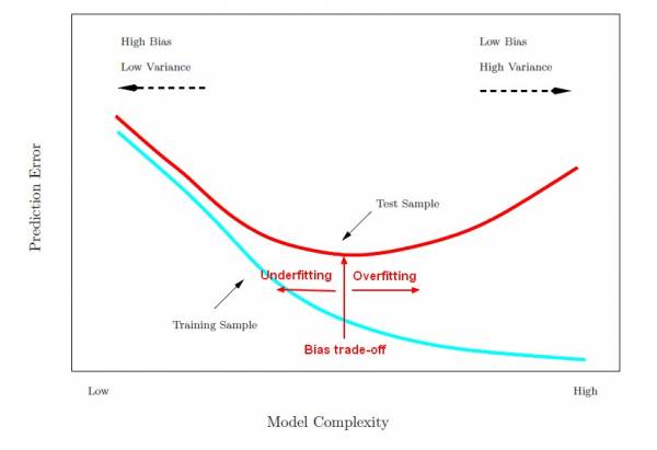
By measuring the evaluation metric at step zero (cold-start), then measuring it again after making adjustments to the model parameters, we learn whether our adjustments led to a better performing model or worse performance. We then know whether to continue making model parameter adjustments in the same direction or in the opposite direction. This is called gradient descent.

Gradient descent methods basically find the slope (i.e., the gradient) of the performance error curve as we progress from one model to the next. As we learned in grade school algebra class, we need two points to find the slope of a curve. Therefore, it is only after we have run and evaluated two models that we will have two performance points — the slope of the curve at the latest point then informs our next choice of model parameter adjustments: either (a) keep adjusting in the same direction as the previous step (if the performance error decreased) to continue descending the error curve; or (b) adjust in the opposite direction (if the performance error increased) to turn around and start descending the error curve.

Note that hill-climbing is the opposite of gradient descent, but essentially the same thing. Instead of minimizing error (a cost function), hill-climbing focuses on maximizing accuracy (a benefit function). Again, we measure the slope of the performance curve from two models, then proceed in the direction of better-performing models. In both cases (hill-climbing and gradient descent), we hope to reach an optimal point (maximum accuracy or minimum error), and then declare that to be the best solution. And that is amazing and satisfying when we remember that we started (as a cold-start) with an initial random guess at the solution.

When our machine learning model has many parameters (which could be thousands for a deep neural network), the calculations are more complex (perhaps involving a multi-dimensional gradient calculation, known as a tensor). But the principle is the same: quantitatively discover at each step in the model-building progression which adjustments (size and direction) are needed in each one of the model parameters in order to progress towards the optimal value of the objective function (e.g., minimize errors, maximize accuracy, maximize goodness of fit, maximize precision, minimize false positives, etc.). In deep learning, as in typical neural network models, the method by which those adjustments to the model parameters are estimated (i.e., for each of the edge weights between the network nodes) is called backpropagation. That is still based on gradient descent.

One way to think about gradient descent, backpropagation, and perhaps all machine learning is this: “Machine Learning is the set of mathematical algorithms that learn from experience. Good judgment comes experience. And experience comes from bad judgment.” In our case, the initial guess for our random cold-start model can be considered “bad judgment”, but then experience (i.e., the feedback from validation metrics such as gradient descent) bring “good judgment” (better models) into our model-building workflow.

Here are ten examples of cold-start problems in data science where the algorithms and techniques of machine learning produce the good judgment in model progression toward the optimal solution:

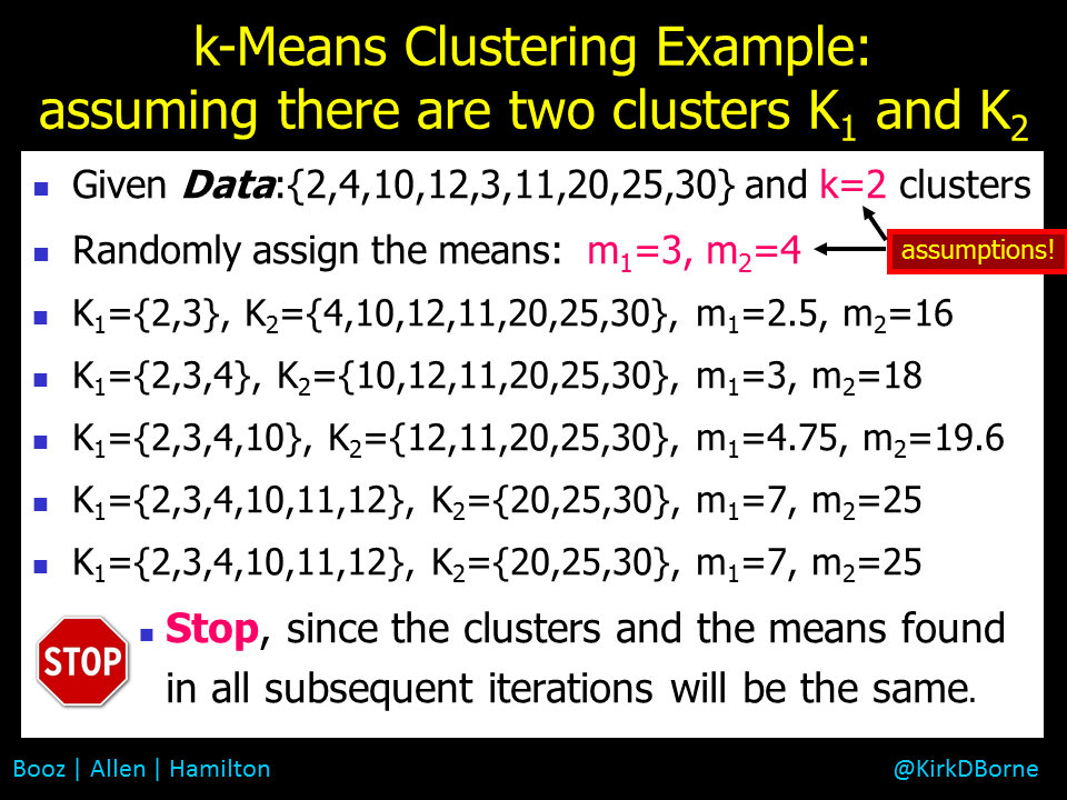
• Clustering analysis (such as K-Means Clustering), where the initial cluster means and the number of clusters are not known in advance (and thus are chosen randomly initially), but the compactness of the clusters can be used to evaluate, iterate, and improve the set of clusters in a progression to the final optimum set of clusters (i.e., the most compact and best separated clusters).
• Neural networks, where the initial weights on the network edges are assigned randomly (a cold-start), but backpropagation is used to iterate the model to the optimal network (with highest classification performance).
• TensorFlow deep learning, which uses the same backpropagation technique of simpler neural networks, but the calculation of the weight adjustments is made across a very high-dimensional parameter space of deep network layers and edge weights using tensors.
• Regression, which uses the sum of the squares of the deviations of the points from the model curve in order to find the best-fit curve. In linear regression, there is a closed-form solution (derivable from the linear least-squares technique). The solution for non-linear regression is not typically a closed-form set of mathematical equations, but the minimization of the sum of the squares of deviations still applies — gradient descent can be used in an iterative workflow to find the optimal curve. Note that K-Means Clustering is actually an example of piecewise regression.
• Nonconvex optimization, where the objective function has many hills and valleys, so that gradient descent and hill-climbing will typically converge only to a local optimum, not to the global optimum. Techniques like genetic algorithms, particle swarm optimization (when the gradient cannot be calculated), and other evolutionary computing methods are used to generate lots of random (cold-start) models and then iterate each of them until you find the global optimum (or until you run out of time and resources, and then pick the best one that you could find). [See my graphic attached below that illustrates a sample use case for genetic algorithms. See also the NOTE below the graphic about Genetic Algorithms, which also applies to other evolutionary algorithms, indicating that these are not machine learning algorithms specifically, but they are actually meta-learning algorithms]
• kNN (k-Nearest Neighbors), which is a supervised learning technique in which the data set itself becomes the model. In other words, the assignment of a new data point to a particular group (which may or may not have a class label or a particular meaning yet) is based simply upon finding which category (group) of existing data points is in the majority when you take a vote of the nearest neighbors to the new data point. The number of nearest neighbors that are to be examined is some number k, which can be initially arbitrary (a cold-start), but then it is adjusted to improve model performance.
• Naive Bayes classification, which applies Bayes theorem to a large data set with class labels on the data items, but for which some combinations of attributes and features are not represented in the training data (i.e., a cold-start challenge). By assuming that the different attributes are mutually independent features of the data items, then one can estimate the posterior likelihood for what the class label should be for a new data item with a feature vector (set of attributes) that is not found in the training data. This is sometimes called a Bayes Belief Network (BBN) and is another example of where the data set becomes the model, where the frequency of occurrence of the different attributes individually can inform the expected frequency of occurrence of different combinations of the attributes.
• Markov modeling (Belief Networks for Sequences) is an extension of BBN to sequences, which can include web logs, purchase patterns, gene sequences, speech samples, videos, stock prices, or any other temporal or spatial or parametric sequence.
• Association rule mining, which searches for co-occurring associations that occur higher than expected from a random sampling of a data set. Association rule mining is yet another example where the data set becomes the model, where no prior knowledge of the associations is known (i.e., a cold-start challenge). This technique is also called Market Basket Analysis, which has been used for simple cold-start customer purchase recommendations, but it also has been used in such exotic use cases as tropical storm (hurricane) intensification prediction.
• Social network (link) analysis, where the patterns in the network (e.g., centrality, reach, degrees of separation, density, cliques, etc.) encode knowledge about the network (e.g., most authoritative or influential nodes in the network), through the application of algorithms like PageRank, without any prior knowledge about those patterns (i.e., a cold-start).

Finally, as a bonus, we mention a special case, Recommender Engines, where the cold-start problem is a subject of ongoing research. The research challenge is to find the optimal recommendation for a new customer or for a new product that has not been seen before. Check out these articles  related to this challenge:

1. The Cold Start Problem for Recommender Systems
2. Tackling the Cold Start Problem in Recommender Systems
3. Approaching the Cold Start Problem in Recommender Systems

We started this article mentioning Confucius and his wisdom. Here is another form of wisdom: https://rapidminer.com/wisdom/ — the RapidMiner Wisdom conference. It is a wonderful conference, with many excellent tutorials, use cases, applications, and customer testimonials. I was honored to be the keynote speaker for their 2018 conference in New Orleans, where I spoke about “Clearing the Fog around Data Science and Machine Learning: The Usual Suspects in Some Unusual Places”. You can find my slide presentation here: KirkBorne-RMWisdom2018.pdf 

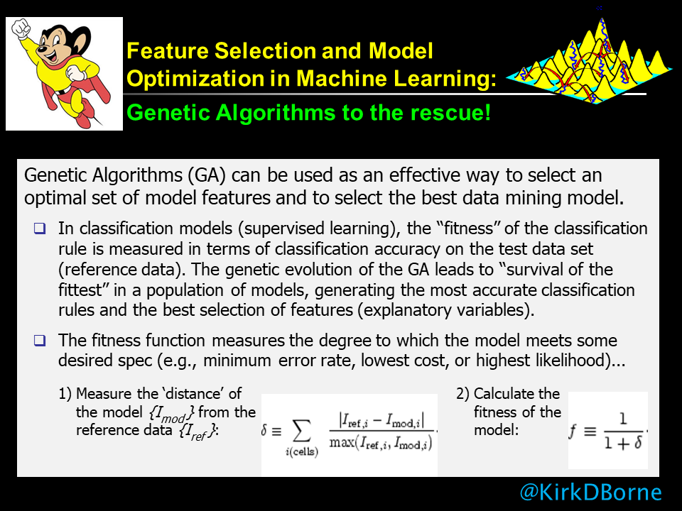
NOTE: Genetic Algorithms (GAs) are an example of meta-learning. They are not machine learning algorithms in themselves, but GAs can be applied across ensembles of machine learning models and tasks, in order to find the optimal model (perhaps globally optimal model) across a collection of locally optimal solutions.