Category Archives: Products

The Power of Graph Databases, Linked Data, and Graph Algorithms

In 2019, I was asked to write the Foreword for the book Graph Algorithms: Practical Examples in Apache Spark and Neo4j, by Mark Needham and Amy E. Hodler. I wrote an extensive piece on the power of graph databases, linked data, graph algorithms, and various significant graph analytics applications. In their wisdom, the editors of the book decided that I wrote “too much”. So, they correctly shortened my contribution by about half in the final published version of my Foreword for the book.

The book is awesome, an absolute must-have reference volume, and it is free (for now, downloadable from Neo4j).
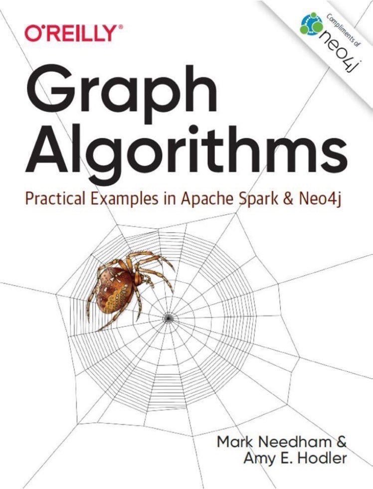
Graph Algorithms book

Now, for the first time, the full unabridged (and unedited) version of my initial contribution as the Foreword for the book is published here. (You should still get the book because it is a fantastic 250-page masterpiece for data scientists!) Any omissions, errors, or viewpoints in the piece below are entirely my own. I publish this in its original form in order to capture the essence of my point of view on the power of graph analytics.

As you read this, just remember the most important message: the natural data structure of the world is not rows and columns, but a graph. And this: perhaps the most powerful node in a graph model for real-world use cases might be “context”. How does one express “context” in a data model? Ahh, that’s the topic for another article. But this might help you get there: https://twitter.com/KirkDBorne/status/1232094501537275904

“All the World’s a Graph”

What do marketing attribution analysis, anti-money laundering, customer journey modeling, safety incident causal factor analysis, literature-based discovery, fraud network analysis, Internet search, the map app on your mobile phone, the spread of infectious diseases, and the theatrical performance of a William Shakespeare play all have in common? No, it is not something as trivial as the fact that all these phrases contain nouns and action verbs! What they have in common is that all these phrases proved that Shakespeare was right when he declared, “All the world’s a graph!”

Okay, the Bard of Avon did not actually say “Graph” in that sentence, but he did say “Stage” in the sentence. However, notice that all the examples mentioned above involve entities and the relationships between them, including both direct and indirect (transitive) relationships — a graph! Entities are the nodes in the graph — these can be people, events, objects, concepts, or places. The relationships between the nodes are the edges in the graph. Therefore, isn’t the very essence of a Shakespearean play the live action portrayal of entities (the nodes) and their relationships (the edges)? Consequently, maybe Shakespeare could have said “Graph” in his famous declaration.

What makes graph algorithms and graph databases so interesting and powerful isn’t the simple relationship between two entities: A is related to B. After all, the standard relational model of databases instantiated these types of relationships in its very foundation decades ago: the ERD (Entity-Relationship Diagram). What makes graphs so remarkably different and important are directional relationships and transitive relationships. In directional relationships, A may cause B, but not the opposite. In transitive relationships, A can be directly related to B and B can be directly related to C, while A is not directly related to C, so that consequently A is transitively related to C.

Because of transitivity relationships, particularly when they are numerous and diverse with many possible relationship (network) patterns and many possible degrees of separation between the entities, the graph model enables discovery of relationships between two entities that otherwise may seem wholly disconnected, unrelated, and difficult (if not impossible) to discover in a relational database. Hence, the graph model can be applied productively and effectively in numerous network analysis use cases.

Consider this marketing attribution use case: person A sees the marketing campaign, person A talks about it on their social media account, person B is connected to person A and sees the comment, and subsequently person B buys the product. From the marketing campaign manager’s perspective, the standard relational model would fail to identify the attribution, since B did not see the campaign and A did not respond to the campaign. The campaign looks like a failure. But it is not a failure — its actual success (and positive ROI) is discovered by the graph analytics algorithm through the transitive relationship between the marketing campaign and the final customer purchase, through an intermediary (entity-in-the-middle)!

Next, consider the anti-money laundering (AML) use case: person A and person C are under suspicion for illicit trafficking. Any interaction between the two (e.g., a financial transaction in a financial database) would be flagged by the authorities, and the interactions would come under great scrutiny. However, if A and C never transact any business together, but instead conduct their financial dealings through a safe, respected, unflagged financial authority B, then who would ever notice the transaction? Well, the graph analytics algorithm would notice! The graph engine would discover that there was a transitive relationship between A and C through the intermediary B (the entity-in-the-middle).

Similar descriptions of the power of graph can be given for the other use cases mentioned in the opening paragraph above, all of which are examples of network analysis through graph algorithms. Each of those cases deeply involves entities (people, objects, events, actions, concepts, and places) and their relationships (touch points, both causal and simple associations). Because of their great interest and power, we highlight two more of those use cases: Internet search and Literature-Based Discovery (LBD).

In Internet search a hyperlinked network (graph-based) algorithm is used by a major search engine to find the central authoritative node across the entire Internet for any given set of search words. The directionality of the edge is most important in this use case since the authoritative node in the network is the one that many other nodes point toward.

LBD is a knowledge network (graph-based) application in which significant discoveries are enabled across the knowledgebase of thousands (and even millions) of research journal articles — the discovery of “hidden knowledge” is only made through the connection between two published research results that may have a large number of degrees of separation (transitive relationships) between them. LBD is being applied to cancer research studies, where the massive semantic medical knowledgebase of symptoms, diagnoses, treatments, drug interactions, genetic markers, short-term results, and long-term consequences may be “hiding” previously unknown cures or beneficial treatments of the most impenetrable cases. The knowledge is already in the network, if only we were to connect the dots to discover it.

The book Graph Algorithms: Practical Examples in Apache Spark and Neo4j is aimed at broadening our knowledge and capabilities around these types of graph analyses, including algorithms, concepts, and practical machine learning applications of the algorithms. From basic concepts to fundamental algorithms, to processing platforms and practical use cases, the authors have compiled an instructive and illustrative guide to the wonderful world of graphs.

Chapter 1 provides a beautiful introduction to graphs, graph analytics algorithms, network science, and graph analytics use cases. In the discussion of power-law distributions, we see again another way that graphs differ from more familiar statistical analyses that assume a normal distribution of properties in random populations. Prepare yourself for some unexpected insights when you realize that power-law distributions are incredibly common in the natural world — graph analytics is a great tool for exploring those scale-free structures and their long tails. By the way, I always love a discussion that mentions the Pareto distribution.

Chapter 2 steps up our graph immersion by introducing us to the many different types of graphs that represent the rich variety of informative relationships that can exist between nodes, including directed and undirected, cyclic and acyclic, trees, and more. If you have always wondered what a DAG was, now you have no more excuses for not knowing. It’s all here. The chapter ends with a quick summary of things to come in greater detail in future chapters, by defining the three major categories of graph algorithms: pathfinding, centrality, and community detection.

Chapter 3 focuses on the graph processing platforms that are mentioned in the subtitle to the book: Apache Spark and Neo4j. In the Apache Spark section, you will find information about the Spark Graph Project, GraphFrames, and Cypher (the graph query language). In the Neo4j section, you will learn about its APOC library: Awesome Procedures On Cypher. Brief instructions on installing these graph engines are included, to prepare you for the use cases and sample applications that are provided later in the book.

Chapters 4, 5, and 6 then dive into the three major graph algorithm categories mentioned earlier. For example, the map app on your mobile phone employs a version of the pathfinding algorithm. Root cause analysis, customer journey modeling, and the spread of infectious diseases are other example applications of pathfinding. Internet search and influencer detection in social networks are example applications of the centrality algorithm. Fraud network analysis, AML, and LBD are example applications of community detection.

Marketing attribution is a use case that may productively incorporate applications of all three graph analytics algorithm categories, depending on the specific question being asked: (1) how did the marketing message flow from source to final action? (pathfinding); (2) was there a dominant influencer who initiated the most ROI from the marketing campaign? (centrality); or (3) is there a community (a set of common personas) that are most responsive to the marketing campaign? (community detection).

Let’s not forget one more example application — a well-conceived theatrical masterpiece will almost certainly be an instantiation of community detection (co-conspirators, love triangles, and all that). That masterpiece will undoubtedly include a major villain or a central hero (representing centrality). Such a masterpiece is probably also a saga (the story of a journey), containing intrigues, strategies, and plots that move ingeniously, methodically, and economically (in three acts or less) toward some climactic ending (thus representing pathfinding).

In Chapter 7, we find many code samples for example applications of graph algorithms, thus rendering all the above knowledge real and useful to the reader. In this manner, the book becomes an instructional tutorial as well as a guide on the side. Putting graph algorithms into practice through these examples is one of the most brilliant contributions of this book — giving you the capability to do it for yourself and to start reaping the rewards of exploring the most natural data structure to describe the world: not rows and columns, but a graph! You will be able to connect the dots that aren’t connected in traditional data structures, build a knowledge graph, explore the graph for insights, and exploit it for value. Let’s put this another way: your graph-powered team will be able to increase the value of your organization’s data assets in ways that others may not have ever imagined. Your team will become graph heroes.

Finally, in Chapter 8, the connection between graph algorithms and machine learning that was implicit throughout the book now becomes explicit. The training data and feature sets that feed machine learning algorithms can now be immensely enriched with tags, labels, annotations, and metadata that were inferred and/or provided naturally through the transformation of your repository of data into a graph of data. Any node and its relationship to a particular node becomes a type of contextual metadata for that particular note. All of that “metadata” (which is simply “other data about your data”) enables rich discovery of shortest paths, central nodes, and communities.

Graph modeling of your data set thus enables more efficient and effective feature extraction and selection (also described in Chapter 8), as the graph exposes the most important, influential, representative, and explanatory attributes to be included in machine learning models that aim to predict a particular target outcome variable as accurately as possible.

When considering the power of graph, we should keep in mind that perhaps the most powerful node in a graph model for real-world use cases might be “context”, including the contextual metadata that we already mentioned. Context may include time, location, related events, nearby entities, and more. Incorporating context into the graph (as nodes and as edges) can thus yield impressive predictive analytics and prescriptive analytics capabilities.

When all these pieces and capabilities are brought together, the graph analytics engine is thereby capable of exploring deep relationships between events, actions, people, and other things across both spatial and temporal (as well as other contextual) dimensions. Consequently, a graph algorithm-powered analysis tool may be called a Spatial-Temporal Analytics Graph Engine (STAGE!). Therefore, if Shakespeare was alive today, maybe he would agree with that logic and would still say “All the world’s a STAGE.” In any case, he would want to read this book to learn how to enrich his stories with deeper insights into the world and with more interesting relationships.

Data Science Training Opportunities

A few years ago, I generated a list of places to receive data science training. That list has become a bit stale. So, I have updated the list, adding some new opportunities, keeping many of the previous ones, and removing the obsolete ones.

Also, here is a thorough, informative, and interesting article that outlines the critical skills needed in order to be a good data scientist: https://www.toptal.com/data-science#hiring-guide

Here are 30 training opportunities that I encourage you to explore:

  1. The Booz Allen Field Guide to Data Science
  2. NYC Data Science Academy
  3. NVIDIA Deep Learning Institute
  4. Metis Data Science Training
  5. Leada’s online analytics labs
  6. Data Science Training by General Assembly
  7. Learn Data Science Online by DataCamp
  8. (600+) Colleges and Universities with Data Science Degrees
  9. Data Science Master’s Degree Programs
  10. Data Analytics, Machine Learning, & Statistics Courses at edX
  11. Data Science Certifications (by AnalyticsVidhya)
  12. Learn Everything About Analytics (by AnalyticsVidhya)
  13. Big Bang Data Science Solutions
  14. CommonLounge
  15. IntelliPaat Online Training
  16. DataQuest
  17. NCSU Institute for Advanced Analytics
  18. District Data Labs
  19. Data School
  20. Galvanize
  21. Coursera
  22. Udacity Nanodegree Program to Become a Data Scientist
  23. Udemy – Data & Analytics
  24. Insight Data Science Fellows Program
  25. The Open Source Data Science Masters
  26. Jigsaw Academy Post Graduate Program in Data Science & Machine Learning
  27. O’Reilly Media Learning Paths
  28. Data Engineering and Data Science Training by Go Data Driven
  29. 18 Resources to Learn Data Science Online (by Simplilearn)
  30. Top Online Data Science Courses to Learn Data Science

Follow Kirk Borne on Twitter @KirkDBorne

Field Guide to Data Science
Learn the what, why, and how of Data Science and Machine Learning here.

Sensor Analytics on Big Data at Micro Scale

We often think of analytics on large scales, particularly in the context of large data sets (“Big Data”). However, there is a growing analytics sector that is focused on the smallest scale. That is the scale of digital sensors — driving us into the new era of sensor analytics.

Small scale (i.e., micro scale) is nothing new in the digital realm. After all, the digital world came into existence as a direct consequence of microelectronics and microcircuits. We used to say in the early years of astronomy big data (which is my background) that the same transistor-based logic microcircuitry that comprises our data storage devices (which are storing massive streams of data) is essentially the same transistor-based logic microcircuitry inside our sensors (which are collecting that data). The latter includes, particularly, the sensors inside digital cameras, consisting of megapixels and even gigapixels. Consequently, there should be no surprise that the two digital data functions (sensing and storing) are intimately connected and that we are therefore drowning in oceans of data.

But, in our rush to crown data “big”, we sometimes may have forgotten that micro-scale component to the story. But not any longer. There is growing movement in the microchip world in new and interesting directions.

I am not only talking about evolutions of the CPU (central processing unit) that we have seen for years: the GPU (graphics processing unit) and the FPGA (field programmable gate array).  We are now witnessing the design, development, and deployment of more interesting application-specific integrated circuits (ASICs), one of which is the TPU (tensor processing unit) which is specifically designed for AI (artificial intelligence) applications. The TPU (as its name suggests) can perform tensor calculations on the chip, in the same way that earlier generation integrated circuits were designed to perform scalar operations (in the CPU) and to perform vector and/or parallel streaming operations (in the GPU).

Speeding the calculations is precisely the goal of these new chips. One that I heard discussed in the context of cybersecurity applications is the BPU (Behavior Processing Unit), designed to detect BOI (behaviors of interest). Whereas the TPU might be detecting persons of interest (POI) or objects of interest in an image, the BOI is looking at patterns in the time series (sequence data) that are indicative of interesting (and/or anomalous) behavioral patterns.

The BOI detector (the BPU) would definitely represent an amplifier to cybersecurity operations, in which the massive volumes of data streaming through our networks and routers are so huge that we never actually capture (and store) all of that data. So we need to detect the anomalous pattern in real-time before a damaging cyber incident occurs!

You can continue reading the long version of this article and learn more about the growing class of new analytics ASIC processors in my article “Sensor Analytics at Micro Scale on the xPU” at the Western Digital DataMakesPossible.com blog site.

Learn more about Machine Learning for Edge Devices at Western Digital here: https://blog.westerndigital.com/machine-learning-edge-devices/

Finally, see what’s cooking in Western Digital’s new Machine Learning Accelerator here: https://blog.westerndigital.com/machine-learning-accelerator-embedded-world-2019/

Brain CPU Chip for AI Acceleration

Brief Guide to xPU for AI Accelerators

Source for graphic: https://www.sigarch.org/a-brief-guide-of-xpu-for-ai-accelerators/

Data Scientist’s Dilemma – The Cold Start Problem

The ancient philosopher Confucius has been credited with saying “study your past to know your future.” This wisdom applies not only to life but to machine learning also. Specifically, the availability and application of labeled data (things past) for the labeling of previously unseen data (things future) is fundamental to supervised machine learning.

Without labels (diagnoses, classes, known outcomes) in past data, then how do we make progress in labeling (explaining) future data? This would be a problem.

A related problem also arises in unsupervised machine learning. In these applications, there is no requirement or presumption regarding the existence of labeled training data — we are essentially parameterizing or characterizing the patterns in the data (e.g., the trends, correlations, segments, clusters, associations).

Many unsupervised learning models can converge more readily and be more valuable if we know in advance which parameterizations are best to choose. If we cannot know that (i.e., because it truly is unsupervised learning), then we would like to know at least that our final model is optimal (in some way) in explaining the data.

In both of these applications (supervised and unsupervised machine learning), if we don’t have these initial insights and validation metrics, then how does such model-building get started and get moving towards the optimal solution?

This challenge is known as the cold-start problem! The solution to the problem is easy (sort of): We make a guess — an initial guess! Usually, that would be a totally random guess.

That sounds so… so… random! How do we know whether it’s a good initial guess? How do we progress our model (parameterizations) from that random initial choice? How do we know that our progression is moving towards more accurate models? How? How? How?

This can be a real challenge. Of course nobody said the “cold start” problem would be easy. Anyone who has ever tried to start a very cold car on a frozen morning knows the pain of a cold start challenge. Nothing can be more frustrating on such a morning. But, nothing can be more exhilarating and uplifting on such a morning than that moment when the engine starts and the car begins moving forward with increasing performance.

The experiences for data scientists who face cold-start problems in machine learning can be very similar to those, especially the excitement when our models begin moving forward with increasing performance.

We will itemize several examples at the end. But before we do that, let’s address the objective function. That is the true key that unlocks performance in a cold-start challenge.  That’s the magic ingredient in most of the examples that we will list.

The objective function (also known as cost function, or benefit function) provides an objective measure of model performance. It might be as simple as the percentage of class labels that the model got right (in a classification model), or the sum of the squares of the deviations of the points from the model curve (in a regression model), or the compactness of the clusters relative to their separation (in a clustering analysis).

The value of the objective function is not only in its final value (i.e., giving us a quantitative overall model performance rating), but its great (perhaps greatest) value is realized in guiding our progression from the initial random model (cold-start zero point) to that final successful (hopefully, optimal) model. In those intermediate steps it serves as an evaluation (or validation) metric.

By measuring the evaluation metric at step zero (cold-start), then measuring it again after making adjustments to the model parameters, we learn whether our adjustments led to a better performing model or worse performance. We then know whether to continue making model parameter adjustments in the same direction or in the opposite direction. This is called gradient descent.

Gradient descent methods basically find the slope (i.e., the gradient) of the performance error curve as we progress from one model to the next. As we learned in grade school algebra class, we need two points to find the slope of a curve. Therefore, it is only after we have run and evaluated two models that we will have two performance points — the slope of the curve at the latest point then informs our next choice of model parameter adjustments: either (a) keep adjusting in the same direction as the previous step (if the performance error decreased) to continue descending the error curve; or (b) adjust in the opposite direction (if the performance error increased) to turn around and start descending the error curve.

Note that hill-climbing is the opposite of gradient descent, but essentially the same thing. Instead of minimizing error (a cost function), hill-climbing focuses on maximizing accuracy (a benefit function). Again, we measure the slope of the performance curve from two models, then proceed in the direction of better-performing models. In both cases (hill-climbing and gradient descent), we hope to reach an optimal point (maximum accuracy or minimum error), and then declare that to be the best solution. And that is amazing and satisfying when we remember that we started (as a cold-start) with an initial random guess at the solution.

When our machine learning model has many parameters (which could be thousands for a deep neural network), the calculations are more complex (perhaps involving a multi-dimensional gradient calculation, known as a tensor). But the principle is the same: quantitatively discover at each step in the model-building progression which adjustments (size and direction) are needed in each one of the model parameters in order to progress towards the optimal value of the objective function (e.g., minimize errors, maximize accuracy, maximize goodness of fit, maximize precision, minimize false positives, etc.). In deep learning, as in typical neural network models, the method by which those adjustments to the model parameters are estimated (i.e., for each of the edge weights between the network nodes) is called backpropagation. That is still based on gradient descent.

One way to think about gradient descent, backpropagation, and perhaps all machine learning is this: “Machine Learning is the set of mathematical algorithms that learn from experience. Good judgment comes experience. And experience comes from bad judgment.” In our case, the initial guess for our random cold-start model can be considered “bad judgment”, but then experience (i.e., the feedback from validation metrics such as gradient descent) bring “good judgment” (better models) into our model-building workflow.

Here are ten examples of cold-start problems in data science where the algorithms and techniques of machine learning produce the good judgment in model progression toward the optimal solution:

  • Clustering analysis (such as K-Means Clustering), where the initial cluster means and the number of clusters are not known in advance (and thus are chosen randomly initially), but the compactness of the clusters can be used to evaluate, iterate, and improve the set of clusters in a progression to the final optimum set of clusters (i.e., the most compact and best separated clusters).
  • Neural networks, where the initial weights on the network edges are assigned randomly (a cold-start), but backpropagation is used to iterate the model to the optimal network (with highest classification performance).
  • TensorFlow deep learning, which uses the same backpropagation technique of simpler neural networks, but the calculation of the weight adjustments is made across a very high-dimensional parameter space of deep network layers and edge weights using tensors.
  • Regression, which uses the sum of the squares of the deviations of the points from the model curve in order to find the best-fit curve. In linear regression, there is a closed-form solution (derivable from the linear least-squares technique). The solution for non-linear regression is not typically a closed-form set of mathematical equations, but the minimization of the sum of the squares of deviations still applies — gradient descent can be used in an iterative workflow to find the optimal curve. Note that K-Means Clustering is actually an example of piecewise regression.
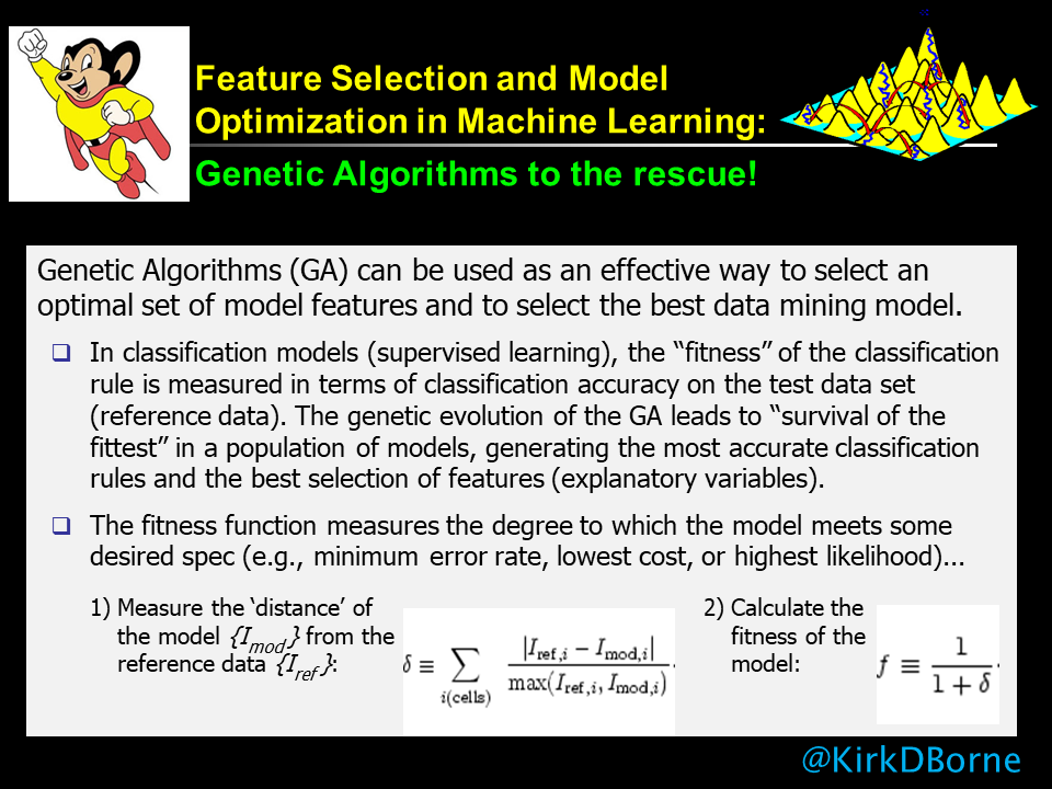
  • Nonconvex optimization, where the objective function has many hills and valleys, so that gradient descent and hill-climbing will typically converge only to a local optimum, not to the global optimum. Techniques like genetic algorithms, particle swarm optimization (when the gradient cannot be calculated), and other evolutionary computing methods are used to generate lots of random (cold-start) models and then iterate each of them until you find the global optimum (or until you run out of time and resources, and then pick the best one that you could find). [See my graphic attached below that illustrates a sample use case for genetic algorithms. See also the NOTE below the graphic about Genetic Algorithms, which also applies to other evolutionary algorithms, indicating that these are not machine learning algorithms specifically, but they are actually meta-learning algorithms]
  • kNN (k-Nearest Neighbors), which is a supervised learning technique in which the data set itself becomes the model. In other words, the assignment of a new data point to a particular group (which may or may not have a class label or a particular meaning yet) is based simply upon finding which category (group) of existing data points is in the majority when you take a vote of the nearest neighbors to the new data point. The number of nearest neighbors that are to be examined is some number k, which can be initially arbitrary (a cold-start), but then it is adjusted to improve model performance.
  • Naive Bayes classification, which applies Bayes theorem to a large data set with class labels on the data items, but for which some combinations of attributes and features are not represented in the training data (i.e., a cold-start challenge). By assuming that the different attributes are mutually independent features of the data items, then one can estimate the posterior likelihood for what the class label should be for a new data item with a feature vector (set of attributes) that is not found in the training data. This is sometimes called a Bayes Belief Network (BBN) and is another example of where the data set becomes the model, where the frequency of occurrence of the different attributes individually can inform the expected frequency of occurrence of different combinations of the attributes.
  • Markov modeling (Belief Networks for Sequences) is an extension of BBN to sequences, which can include web logs, purchase patterns, gene sequences, speech samples, videos, stock prices, or any other temporal or spatial or parametric sequence.
  • Association rule mining, which searches for co-occurring associations that occur higher than expected from a random sampling of a data set. Association rule mining is yet another example where the data set becomes the model, where no prior knowledge of the associations is known (i.e., a cold-start challenge). This technique is also called Market Basket Analysis, which has been used for simple cold-start customer purchase recommendations, but it also has been used in such exotic use cases as tropical storm (hurricane) intensification prediction.
  • Social network (link) analysis, where the patterns in the network (e.g., centrality, reach, degrees of separation, density, cliques, etc.) encode knowledge about the network (e.g., most authoritative or influential nodes in the network), through the application of algorithms like PageRank, without any prior knowledge about those patterns (i.e., a cold-start).

Finally, as a bonus, we mention a special case, Recommender Engines, where the cold-start problem is a subject of ongoing research. The research challenge is to find the optimal recommendation for a new customer or for a new product that has not been seen before. Check out these articles  related to this challenge:

  1. The Cold Start Problem for Recommender Systems
  2. Tackling the Cold Start Problem in Recommender Systems
  3. Approaching the Cold Start Problem in Recommender Systems

We started this article mentioning Confucius and his wisdom. Here is another form of wisdomhttps://rapidminer.com/wisdom/ — the RapidMiner Wisdom conference. It is a wonderful conference, with many excellent tutorials, use cases, applications, and customer testimonials. I was honored to be the keynote speaker for their 2018 conference in New Orleans, where I spoke about “Clearing the Fog around Data Science and Machine Learning: The Usual Suspects in Some Unusual Places”. You can find my slide presentation here: KirkBorne-RMWisdom2018.pdf 

NOTE: Genetic Algorithms (GAs) are an example of meta-learning. They are not machine learning algorithms in themselves, but GAs can be applied across ensembles of machine learning models and tasks, in order to find the optimal model (perhaps globally optimal model) across a collection of locally optimal solutions.

Definitive Guides to Data Science and Analytics Things

The Definitive Guide to anything should be a helpful, informative road map to that topic, including visualizations, lessons learned, best practices, application areas, success stories, suggested reading, and more.  I don’t know if all such “definitive guides” can meet all of those qualifications, but here are some that do a good job:

  1. The Field Guide to Data Science (big data analytics by Booz Allen Hamilton)
  2. The Data Science Capability Handbook (big data analytics by Booz Allen Hamilton)
  3. The Definitive Guide to Becoming a Data Scientist (big data analytics)
  4. The Definitive Guide to Data Science – The Data Science Handbook (analytics)
  5. The Definitive Guide to doing Data Science for Social Good (big data analytics, data4good)
  6. The Definitive Q&A Guide for Aspiring Data Scientists (big data analytics, data science)
  7. The Definitive Guide to Data Literacy for all (analytics, data science)
  8. The Data Analytics Handbook Series (big data, data science, data literacy by Leada)
  9. The Big Analytics Book (big data, data science)
  10. The Definitive Guide to Big Data (analytics, data science)
  11. The Definitive Guide to the Data Lake (big data analytics by MapR)
  12. The Definitive Guide to Business Intelligence (big data, business analytics)
  13. The Definitive Guide to Natural Language Processing (text analytics, data science)
  14. A Gentle Guide to Machine Learning (analytics, data science)
  15. Building Machine Learning Systems with Python (a non-definitive guide) (data analytics)
  16. The Definitive Guide to Data Journalism (journalism analytics, data storytelling)
  17. The Definitive “Getting Started with Apache Spark” ebook (big data analytics by MapR)
  18. The Definitive Guide to Getting Started with Apache Spark (big data analytics, data science)
  19. The Definitive Guide to Hadoop (big data analytics)
  20. The Definitive Guide to the Internet of Things for Business (IoT, big data analytics)
  21. The Definitive Guide to Retail Analytics (customer analytics, digital marketing)
  22. The Definitive Guide to Personalization Maturity in Digital Marketing Analytics (by SYNTASA)
  23. The Definitive Guide to Nonprofit Analytics (business intelligence, data mining, big data)
  24. The Definitive Guide to Marketing Metrics & Analytics
  25. The Definitive Guide to Campaign Tagging in Google Analytics (marketing, SEO)
  26. The Definitive Guide to Channels in Google Analytics (SEO)
  27. A Definitive Roadmap to the Future of Analytics (marketing, machine learning)
  28. The Definitive Guide to Data-Driven Attribution (digital marketing, customer analytics)
  29. The Definitive Guide to Content Curation (content-based marketing, SEO analytics)
  30. The Definitive Guide to Collecting and Storing Social Profile Data (social big data analytics)
  31. The Definitive Guide to Data-Driven API Testing (analytics automation, analytics-as-a-service)
  32. The Definitive Guide to the World’s Biggest Data Breaches (visual analytics, privacy analytics)

Follow Kirk Borne on Twitter @KirkDBorne

4_book_image-6fd6043b69f0bb051f45055c9481cccc

Just-in-Time Supply Chain Management with Data Analytics

A common phrase in SCM (Supply Chain Management) is Just-In-Time (JIT) inventory. JIT refers to a management strategy in which raw materials, products, or services are delivered to the right place, at the right time, as demand requires. This has always been an excellent business goal, but the power to excel at JIT inventory management is now improving dramatically with the increased use of data analytics across the supply chain.

In the article “Operational Analytics and Droning About Big Data“, we discussed two examples of JIT: (1) a just-in-time supply replenishment system for human bases on the Moon, and (2) the proposal by Amazon to use drones to deliver products to your front door “just in time”! The Internet of Things will almost certainly generate similar use cases and benefits.

Descriptive analytics (hindsight) tells you what has already happened in your supply chain. If there was a deficiency or problem somewhere, then you can react to that event. But, that is “old school” supply chain management. Modern analytics is predictive (foresight), allowing you to predict where the need will occur (in advance) so that you can proactively deliver products and services at the point of need, just in time.

The next advance in analytics is prescriptive (insight), which uses optimization techniques (from operations research) in combination with insights and knowledge of your business (systems, processes, and resources) in order to optimize your delivery systems, for the best possible outcome (greater sales, fewer losses, reduced inventory, etc.). Just-in-time supply chain management then becomes something more than a reality — it now becomes an enabler of increased efficiency and productivity.

Many more examples of use cases in the manufacturing and retail industries (and elsewhere) where just-in-time analytics is important (and what you can do about it) have been enumerated by the fast Automatic Modeling folks from Soft10, Inc. Check out their fast predictive analytics products at http://soft10ware.com/.

(Read more about these ideas at: https://www.linkedin.com/pulse/supply-chain-data-analytics-jit-legit-kirk-borne)

Follow Kirk Borne on Twitter @KirkDBorne


Drilling Through Data Silos with Apache Drill

Enterprise data collections are typically stored in silos belonging to different business divisions. Sometimes these silos belong to different projects within the same division. These silos may be further segmented by services/products and functions. Silos (which stifle data-sharing and innovation) are often identified as a primary impediment (both practically and culturally) to business progress and thus they may be the cause of numerous difficulties. For example, streamlining important business processes are rendered more challenging, ranging from compliance to data discovery. But, breaking down the silos may not be so easy to accomplish. In fact, it is often infeasible due to ownership issues, governance practices, and regulatory concerns.

Big Data silos create additional complications including data duplication (and associated increased costs), complicated data replication solutions, high data latency, and data quality concerns, not to mention being an enabler of the real problematic situation where your data repositories could hold different versions of the truth. The silos also put a limit on business intelligence (discovery and actionable insights). As big data best practices rise above the hype and noise, we now know that actionable value is more easily extracted when multiple data sets can be integrated and viewed holistically.

Data analysts naturally want to break down silos to combine data from multiple data sources. Unfortunately, this can create its own bottleneck: a complex integration labyrinth—which is costly to maintain, rarely performs well, and can’t be guaranteed to provide consistent results.

In response, many companies have deployed Apache Hadoop to address the problem of segregated data. Hadoop enables multiple types of data to be directly processed in place, and it fully supports data integration from multiple sources across different data storage technologies.

Organizations that use Hadoop are finding additional benefits with Apache Drill, which is the open source version of Google’s Dremel system…

(continue reading here https://www.mapr.com/blog/drive-innovation-breaking-down-data-silos-apache-drill)

Follow Kirk Borne on Twitter @KirkDBorne

Clear and Obvious Analytics for Clear and Present Dangers

Not every industry has found their clear and obvious applications of big data analytics. But the clear and present dangers of risk and fraud in financial transactions demand fast predictive modeling. Precisely because we live in the ubiquitous digital era, where most business (and non-business) transactions are rarely (if ever) in analog form and those transactions no longer move at the pace of humans (but at the speed of light), consequently the volume of digital signals as well as lurking dangers is enormous.

Digital signals (from sensors everywhere in our operational business systems) carry transactional information (what happened to what?), as well as metadata (descriptors) and analytics information (data-encoded knowledge and insights).  These analytics can be behavioral (providing insights into the interests, intentions, and preferences of the actors in a given transaction) as well as functional (providing insights into the actions or events associated with the transaction).

Behavioral analytics is developing into a major component of digital marketing, as firms seek to sell, cross-sell, and up-sell their products to the right customer at the right time.  Behavioral analytics is also critical in risk mitigation of all sorts: financial, cybersecurity, health (individual and population), supply chain, machine performance, and so on.

Here are 10 examples of where fast predictive analytics can play a vital role in most industries (with a focus on financial):

  1. Predict credit risk and fraud in real-time!
  2. Use Social Media for deeper understanding (likes and dislikes) of your customers.
  3. Personalize customer interactions in real-time, across multiple channels.
  4. Stop improper insurance payments before claims are paid!
  5. Spot insurance rate evasion tactics during the quote process – before you issue a policy!
  6. Predict High Health Risk versus Low Health Risk to better manage healthcare decision-making.
  7. Generate better predictive models of health, car, and home insurance eligibility fraud, underwriting fraud, and improper payments.
  8. Spot adversarial and anomalous behavior in cyber networks – stop the data breach or illegal funds transfer before it happens!
  9. Eliminate your Supply Chain hiccups – move the right products to the right locations in the right quantities – and at the right time!
  10. Make better business decisions regarding merchandising, demand forecasting, and pricing – don’t leave money on the table, or products in your warehouse.

Let us look a little more closely at the financial services industry…

One of the common conditions in traditional financial services (including home, health, and auto insurance) has been the “pay and chase” — i.e., you make the payment to the claimant, and then (after making the payment) you find out that the claim is fraudulent, thus beginning the chase to get your money back.

The new world of predictive modeling and advanced analytics allows for a new mantra in the financial and insurance industries: “Do Not Pay!” — i.e., you do not pay the claim until you have analyzed its likelihood for claim fraud, extraordinary financial risk, or payment anomalies (e.g., duplicate payments).

Predictive analytics modeling delivers a better financial risk posture for your organization than the “pay and chase”. With access to greater and more diverse data sources, it is now possible to develop better models of your customers’ credit risk regardless of the industry. This is certainly true in the financial services industry where there is so much data available: credit scores, credit history, court records, tax records, health records, insurance claims, and more. There is no excuse for not examining as much “public data” as you can in conjunction with other data sources that are available to you internally within your organization. Moderate outlays of your organization’s funds that are incurred in acquiring access to diverse external data sources should be offset by the savings accrued by “not sending your funds out the door” erroneously (either to intentional fraudsters or in unintentional duplicate claims).

An analytics-driven predictive model can predict fraud more efficiently (with fast automatic statistical software packages) and more effectively (with higher precision and higher recall: fewer false positives and false negatives) than traditional business processes. A good predictive analytics model should: (a) detect claims that “smell funny”, (b) prevent the “pay and chase” mode of operations, and (c) stop claims fraud abruptly by empowering a “do not pay” mode of operations. Predictive analytics modeling should aim to satisfy the following business requirements:

  • Detect and prevent both opportunistic and professional fraud throughout the claims process.
  • Detect underwriting fraud, to prevent premium leakage at the point of sale and renewal.
  • Spot rate evasion tactics during the quote process – before you issue a policy.

Many more examples of use cases in the financial services industry (and elsewhere) where fast predictive analytics is important (and what you can do about it) have been expertly enumerated by the fast statistical modeling folks from Soft10, Inc. Check out their fast analytics products (including the Instant Online Overbilling Claims Detector) at http://soft10ware.com/.

Follow Kirk Borne on Twitter @KirkDBorne

Where to get your Data Science Training or Apprenticeship

I am frequently asked for suggestions regarding academic institutions, professional organizations, or MOOCs that provide Data Science training.  The following list will be updated occasionally (LAST UPDATED: 2018 March 29) .

Also, be sure to check out The Definitive Q&A for Aspiring Data Scientists and the story of my journey from Astrophysics to Data Science. If the latter story interests you, then here are a couple of related interviews: “Data Mining at NASA to Teaching Data Science at GMU“, and “Interview with Leading Data Science Expert“.

Here are a few places to check out:

  1. The Booz Allen Field Guide to Data Science
  2. Do you have what it takes to be a Data Scientist? (get the Booz Allen Data Science Capability Handbook)
  3. http://www.thisismetis.com/explore-data-science-online-training (formerly exploredatascience.com at Booz-Allen)
  4. http://www.thisismetis.com/
  5. https://www.teamleada.com/
  6. MapR Academy (offering Free Hadoop, Spark, HBase, Drill, Hive training and certifications at MapR)
  7. Data Science Apprenticeship at DataScienceCentral.com
  8. (500+) Colleges and Universities with Data Science Degrees
  9. List of Machine Learning Certifications and Best Data Science Bootcamps
  10. NYC Data Science Academy
  11. NCSU Institute for Advanced Analytics
  12. Master of Science in Analytics at Bellarmine University
  13. http://www.districtdatalabs.com/ (District Data Labs)
  14. http://www.dataschool.io/
  15. http://www.persontyle.com/school/ 
  16. http://www.galvanize.it/education/#classes (formerly Zipfian Academy) includes http://www.galvanizeu.com/ (Data Science, Statistics, Machine Learning, Python)
  17. https://www.coursera.org/specialization/jhudatascience/1
  18. https://www.udacity.com/courses#!/data-science 
  19. https://www.udemy.com/courses/Business/Data-and-Analytics/
  20. http://insightdatascience.com/ 
  21. Data Science Master Classes (at Datafloq)
  22. http://datasciencemasters.org
  23. http://www.jigsawacademy.com/
  24. https://intellipaat.com/
  25. http://www.athenatechacademy.com/ (Hadoop training, and more)
  26. O’Reilly Media Learning Paths
  27. http://www.godatadriven.com/training.html
  28. Courses for Data Pros at Microsoft Virtual Academy
  29. 18 Resources to Learn Data Science Online (by Simplilearn)
  30. Learn Everything About Analytics (by AnalyticsVidhya)
  31. Data Science Masters Degree Programs

DataMiningTagCloudTagxedoWordCloud

Follow Kirk Borne on Twitter @KirkDBorne

Variety is the Spice of Life for Data Scientists

“Variety is the spice of life,” they say.  And variety is the spice of data also: adding rich texture and flavor to otherwise dull numbers. Variety ranks among the most exciting, interesting, and challenging aspects of big data.  Variety is one of the original “3 V’s of Big Data” and is frequently mentioned in Big Data discussions, which focus too much attention on Volume.

A short conversation with many “old school technologists” these days too often involves them making the declaration: We’ve always done big data.”  That statement really irks me… for lots of reasons.  I summarize in the following article some of those reasons:  “Today’s Big Data is Not Yesterday’s Big Data.” In a nutshell, those statements focus almost entirely on Volume, which is really missing the whole point of big data (in my humble opinion)… here comes the Internet of Things… hold onto your bits!

The greatest challenges and the most interesting aspects of big data appear in high-Velocity Big Data (requiring fast real-time analytics) and high-Variety Big Data (enabling the discovery of interesting patterns, trends, correlations, and features in high-dimensional spaces). Maybe because of my training as an astrophysicist, or maybe because scientific curiosity is a natural human characteristic, I love exploring features in multi-dimensional parameter spaces for interesting discoveries, and so should you!

Dimension reduction is a critical component of any solution dealing with high-variety (high-dimensional) data. Being able to sift through a mountain of data efficiently in order to find the key predictive, descriptive, and indicative features of the collection is a fundamental required data science capability for coping with Big Data.

Identifying the most interesting dimensions of the data is especially valuable when visualizing high-dimensional data. There is a “good news, bad news” perspective here. First, the bad news: the human capacity for seeing multiple dimensions is very limited: 3 or 4 dimensions are manageable; and 5 or 6 dimensions are possible; but more dimensions are difficult-to-impossible to assimilate. Now for the good news: the human cognitive ability to detect patterns, anomalies, changes, or other “features” in a large complex “scene” surpasses most computer algorithms for speed and effectiveness. In this case, a “scene” refers to any small-n projection of a larger-N parameter space of variables.

In data visualization, a systematic ordered parameter sweep through an ensemble of small-n projections (scenes) is often referred to as a “grand tour”, which allows a human viewer of the visualization sequence to see quickly any patterns or trends or anomalies in the large-N parameter space. Even such “grand tours” can miss salient (explanatory) features of the data, especially when the ratio N/n is large. Consequently, a data analytics approach that combines the best of both worlds (machine vision algorithms and human perception) will enable efficient and effective exploration of large high-dimensional data.

One such approach is to use statistical and machine learning techniques to develop “interestingness metrics” for high-variety data sets.  As such algorithms are applied to the data (in parameter sweeps or grand tours), they can discover and then present to the data end-user the most interesting and informative features (or combinations of features) in high-dimensional data: “Numbers are powerful, especially in interesting combinations.”

The outcomes of such exploratory data analyses are even more enhanced when the analytics tool ranks the output models (e.g., the data’s “most interesting parameters”) in order of significance and explanatory power (i.e., their ability to “explain” the complex high-dimensional patterns in the data).  Soft10’s “automatic statistician” Dr. Mo is a fast predictive analytics software package for exploring complex high-dimensional (high-variety) data.  Dr. Mo’s proprietary modeling and analytics techniques have been applied across many application domains, including medicine and health, finance, customer analytics, target marketing, nonprofits, membership services, and more. Check out Dr. Mo at http://soft10ware.com/ and read more herehttp://soft10ware.com/big-data-complexity-requires-fast-modeling-technology/

Kirk Borne is a member of the Soft10, Inc. Board of Advisors.

Follow Kirk Borne on Twitter @KirkDBorne